Calculus the right way

Calculus is the branch of mathematics that studies continuous change.

it has two major branches, differential calculus and integral calculus.

Calculus is the mathematical backbone for solving problems in which variable quantities change with time or another reference value.

Calculus is fundamental to many scientific disciplines including physics, engineering, and economics.

Differential calculus

The derivative is a fundamental tool that quantifies the sensitivity to change of a function’s output with respect to its input. The derivative of a function of a single variable at a chosen input value, when it exists, is the slope of the tangent line to the graph of the function at that point.

The tangent line is the best linear approximation of the function near that input value. The derivative is often described as the instantaneous rate of change, the ratio of the instantaneous change in the dependent variable to that of the independent variable. The process of finding a derivative is called differentiation.

Leibniz’s notation:

\[\frac{dy}{dx}\]

symbols dx and dy to represent infinitely small (or infinitesimal) increments of x and y, respectively, just as Δx and Δy represent finite increments of x and y, respectively

Consider y as a function of a variable x, or y = f(x). If this is the case, then the derivative of y with respect to x, which later came to be viewed as the limit.

\[\lim_{\Delta x \to 0} \frac{\Delta y}{\Delta x} = \lim_{\Delta x \to 0} \frac{f(x+\Delta x) - f(x)}{\Delta x}\]

was, according to Leibniz, the quotient of an infinitesimal increment of y by an infinitesimal increment of x, or

\[\frac{dy}{dx} = f'(x)\]

Single Variable Calculus

Single variable calculus is the study of functions of one real variable, centering on limits, differentiation, and integration. It explores how a single input value x changes an output value f(x), measuring instantaneous rates of change and total accumulation.

It is the foundation for multivariable calculus and is used in many fields including physics, engineering, and economics.

Core Concepts

• Limits: The foundation of calculus; describes the behavior of a function as its input approaches a specific value.

• Derivatives: Measures the instantaneous rate of change or the slope of the tangent line to a function’s curve at any given point.

• Integrals: Measures the accumulation of quantities, interpreted geometrically as the net signed area underneath a function’s graph.

• Infinite Series: The summation of an infinite sequence of numbers, often used to approximate complex continuous functions.

\[y = f(x)\]

---

Single Variable Calculus 18.01SC | Fall 2010 | Undergraduate

What is Derivative?

• geometric interpretation: slope of the tangent line to the curve at a point
• physical interpretation: instantaneous rate of change

How to differentiate any function we know?

GEOMETRIC APPROACH: Find the tangent to $y=f(x)$ at point $P = (x_0, y_0)$

The line equation is:

proof:

• Let (x,y) be any arbitrary point on a straight line.
• Let m be the slope (steepness) of the line.
• Let c be the y-intercept, which means the line crosses the vertical y-axis at the point (0,c).

Slope: slope ($m$) is the change in $y$ over the change in $x$. It tells us how steep a line is and whether it rises or falls as $x$ increases.

The slope ($m$) between any two points ($x_1, y_1$) and ($x_2, y_2$) on a line is:

\[m = \frac{y_2 - y_1}{x_2 - x_1}\]

we know one point on the line is $(0, c)$ as (x₁, y₁) and another point is (x, y) as ($x_2, y_2$):

\[m = \frac{y - c}{x - 0}\]

Since $m = \frac{y - c}{x - 0}$ , we can solve for $y$:

\[y = mx + c\]

Two-point form of line equation:

\[\frac{y - y_1}{x - x_1} = \frac{y_2 - y_1}{x_2 - x_1}\]

proof:

• Let $P(x, y)$ be any arbitrary point on a straight line.
• Let $P_1(x_1, y_1)$ and $P_2(x_2, y_2)$ be two distinct fixed points on a straight line.

Using the two known points $P_1(x_1, y_1)$ and $P_2(x_2, y_2)$, we can find the slope $m$ of the line:

\[m = \frac{y_2 - y_1}{x_2 - x_1} \tag{1}\]

Because the line is straight, the slope between $P_1(x_1, y_1)$ and the general point $P(x,y)$ must be identical to $m$:

\[\frac{y - y_1}{x - x_1} = m \tag{2}\]

From (1) and (2):

\[\frac{y - y_1}{x - x_1} = \frac{y_2 - y_1}{x_2 - x_1} \tag{3}\]

This is the two-point form of the line equation.

\[y - y_1 = \frac{y_2 - y_1}{x_2 - x_1}(x - x_1) \tag{4}\]

So, to draw a tangent line to a curve at a point, we need to find the slope of the tangent line at that point.

tangent line: \(y - y_0 = m(x - x_0)\)

point of tangency: \(y_0 = f(x_0)\)

slope: \(m = f'(x_0)\)

it’s all about slope!

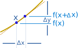
where $\Delta x$ is the change in $x$ and $\Delta y$ is the change in $y$. i.e. $\Delta f$

then slope of the tangent line (m) is: \(m = \lim_{\Delta x \to 0} \frac{\Delta f}{\Delta x} \text{ slope of secant line as } \Delta x \to 0\)

the point P is $(x_0, f(x_0))$ and point Q is $(x_0 + \Delta x, f(x_0 + \Delta x))$

Derivate (slope of tangent line):

slope = change in y / change in x = \(\frac{\Delta y} {\Delta x}\)

x changes from \(x\) to \(x + \Delta x\)

y changes from \(f(x)\) to \(f(x + \Delta x)\)

• fill in the slope formula:

\[\frac{\Delta y}{\Delta x} = \frac{f(x + \Delta x) - f(x)}{x + \Delta x - x}\] \[= \frac{f(x + \Delta x) - f(x)}{\Delta x} \to \text{ slope of secant line}\]

as $\Delta x \to 0$, the secant line approaches the tangent line.

Therefore, the derivative is:

\[f'(x) = \lim_{\Delta x \to 0} \frac{f(x + \Delta x) - f(x)}{\Delta x} \to \text{slope of the tangent line at } x\]

This gives the slope of the tangent line to the curve at the point ((x,f(x))).

---

Leibniz’s Notation

Instead of using the notation (f’(x)), Gottfried Wilhelm Leibniz introduced the notation

\[\frac{dy}{dx}\]

If (x) changes by a very small amount (dx), then the corresponding change in (y) is denoted by (dy).

The derivative is written as

\[\frac{dy}{dx}\]

Historically, Leibniz viewed (dx) and (dy) as infinitesimally small changes in (x) and (y). In modern calculus, the derivative is rigorously defined using the limit

\[\frac{dy}{dx} = \lim_{\Delta x\to0} \frac{\Delta y}{\Delta x}\]

Since

\[\Delta y = f(x + \Delta x) - f(x)\]

we obtain

\[\frac{dy}{dx} = \lim_{\Delta x\to0} \frac{f(x+\Delta x)-f(x)}{\Delta x}\]

Therefore,

\[\boxed{\frac{dy}{dx} = f'(x)}\]

Both notations represent exactly the same derivative.

---

Differentials

Once the derivative is known, we define the differential (dy) by

\[dy = f'(x) dx\]

Here,

• (dx) represents an infinitesimal change in the independent variable.
• (dy) is the corresponding differential of (y).

For a small change in (x),

\[\Delta y = f(x+\Delta x)-f(x)\]

while

\[dy = f'(x) dx\]

The differential (dy) is a linear approximation of the actual change (\Delta y).

Thus,

\[\Delta y \approx dy\]

whenever the change in (x) is sufficiently small.

This approximation becomes more accurate as

\[dx \to 0\]

The relationship

\[dy = f'(x) dx\]

is one of the most useful ideas in calculus and forms the basis of applications such as error estimation, linear approximation, optimization, differential equations, and much more.