Sorting
A Sorting Algorithm is an algorithm that puts elements of a list into an order. The most frequently used orders are numerical order and lexicographical order, and either ascending or descending.
Efficient sorting is important for optimizing the efficiency of other algorithms (such as search and merge algorithms) that require input data to be in sorted lists. Sorting is also often useful for canonicalizing data and for producing human-readable output.
Sorting Algorithm
What is Selection Sort?
Selection Sort is a simple, in-place, comparison-based sorting algorithm. It works by repeatedly finding the minimum (or maximum) element from the unsorted portion of the list and placing it at the beginning (or end) of the sorted portion.
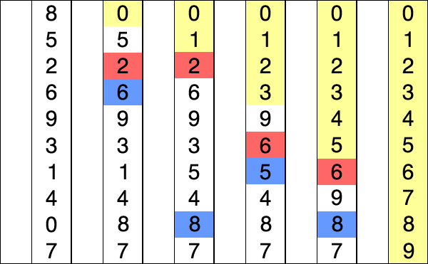
How does it work?
-
Selection: The algorithm scans the unsorted part of the array to find the smallest (or largest, for descending) element.
-
Swapping: It swaps this smallest element with the first element of the unsorted part.
-
Expansion: The boundary of the sorted portion moves one step to the right, and the process repeats for the remaining unsorted elements.
-
Completion: This continues until the entire array is sorted, typically requiring n-1 passes for an array of size n.
What is its time and space complexity?
-
Time Complexity: $O(n^2)$ for best, average, and worst-case scenarios. Because the algorithm must scan the remaining unsorted part entirely to find the minimum in each pass, it is not adaptive to already sorted data.
-
Space Complexity: $O(1)$ , as it only requires a constant amount of extra memory for temporary variables used during swapping
What are its key characteristics?
- In-Place: It modifies the original array directly without needing extra storage.
- Unstable: By default, it may change the relative order of equal elements because it swaps non-adjacent elements.
- Minimal Swaps: While it has poor time complexity, it performs only $O(n)$ swaps, making it useful for memory environments where write operations are costly (e.g., Flash memory or EEPROM).
When should you use it?
- Small Data Sets: Where simplicity is preferred over peak efficiency.
- Costly Memory Writes: When minimizing the number of write operations is more important than reducing comparisons.
- Educational Purposes: Its straightforward logic makes it an ideal introductory algorithm for learning sorting fundamentals.
Class: Sorting algorithm
Data structure: ArrayWorst-case performance:
O(n²)comparisonsO(n)swapsBest-case performance:
O(n²)comparisonsO(1)swapAverage performance:
O(n²)comparisonsO(n)swapsWorst-case space complexity:
O(1)auxiliaryOptimal: No
What is Bubble Sort?
Bubble Sort is a simple, comparison-based algorithm where each pair of adjacent elements is compared and swapped if they are in the wrong order. This process repeats until the largest elements “bubble up” to their correct positions at the end of the list.
How does it work?
- Compare Adjacent Elements: Start at the beginning of the list and compare the first two elements.
- Swap: If the first element is larger than the second, swap them.
- Move Forward: Move to the next pair and repeat the comparison/swap until the end of the list is reached.
- Complete the Pass: After the first pass, the largest element is guaranteed to be at the final position.
- Repeat: Repeat the entire process for the remaining unsorted elements until a full pass occurs without any swaps.
What is its time and space complexity?
- Best Case: $O(n)$ – Occurs when the array is already sorted (requires an optimized version that stops if no swaps are made).
- Average Case: $O(n^2)$ – Occurs when elements are in random order.
- Worst Case: $O(n^2)$ – Occurs when the array is sorted in reverse order.
- Space Complexity: $O(1)$ – It is an in-place algorithm, requiring no extra storage.
What are its key characteristics?
- Stable: It maintains the relative order of elements with equal values.
- In-Place: It only requires a constant amount of additional memory space.
- Simple: It is one of the easiest algorithms to understand and write, making it a popular teaching tool.
- High Overhead: It performs a large number of swaps compared to other algorithms like Insertion Sort.
When should you use it?
- Educational Purposes: Ideal for introducing the concept of sorting and algorithmic logic to beginners.
- Very Small Datasets: Can be used when the dataset size is so small that complexity doesn’t impact performance.
- Nearly Sorted Data: Useful if you only need to swap one or two elements that are slightly out of place.
- Detecting a Sorted List: The optimized version is very efficient at simply confirming if a list is already sorted.
Do you want to see how Selection Sort compares to these two?
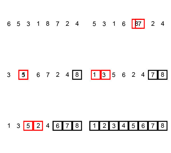
How does a step-by-step example look?
1
2
3
4
5
6
7
8
9
10
11
12
13
14
15
16
17
18
19
Take an array of numbers "5 1 4 2 8"

First pass
( 5 1 4 2 8 ) → ( 1 5 4 2 8 ), Here, algorithm compares the first two elements, and swaps since 5 > 1.
( 1 5 4 2 8 ) → ( 1 4 5 2 8 ), Swap since 5 > 4
( 1 4 5 2 8 ) → ( 1 4 2 5 8 ), Swap since 5 > 2
( 1 4 2 5 8 ) → ( 1 4 2 5 8 ), Now, since these elements are already in order (8 > 5), algorithm does not swap them.

Second pass
( 1 4 2 5 8 ) → ( 1 4 2 5 8 )
( 1 4 2 5 8 ) → ( 1 2 4 5 8 ), Swap since 4 > 2
( 1 2 4 5 8 ) → ( 1 2 4 5 8 )
( 1 2 4 5 8 ) → ( 1 2 4 5 8 )

Third pass
( 1 2 4 5 8 ) → ( 1 2 4 5 8 )
( 1 2 4 5 8 ) → ( 1 2 4 5 8 )
( 1 2 4 5 8 ) → ( 1 2 4 5 8 )
( 1 2 4 5 8 ) → ( 1 2 4 5 8 )
Class: Sorting algorithm
Data structure: ArrayWorst-case performance:
O(n²)comparisonsO(n²)swapsBest-case performance:
O(n)comparisonsO(1)swapsAverage performance:
O(n²)comparisonsO(n²)swapsWorst-case space complexity:
O(n)totalO(1)auxiliaryOptimal: No
What is Insertion Sort?
Insertion sort is a simple, intuitive sorting algorithm that builds a final sorted list one element at a time. It is often compared to the way a person might sort a hand of playing cards: you pick one card at a time and insert it into its correct position relative to the cards you are already holding.
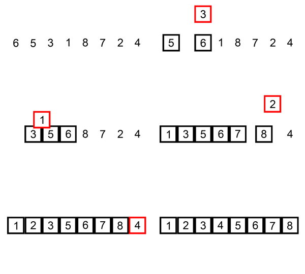

Becomes

How does it work?
The algorithm virtually splits the input array into two parts: a sorted portion (on the left) and an unsorted portion (on the right).
- Initialize: Assume the first element is already sorted.
- Pick a Key: Move to the next element (the “key”) from the unsorted part.
- Compare and Shift: Compare this key with the elements in the sorted portion from right to left. If a sorted element is larger than the key, shift it one position to the right.
- Insert: Once you find the correct spot-where the element to the left is smaller than or equal to the key-insert the key into that position.
- Repeat: Continue this process until every element from the unsorted part has been moved to its correct position.
What is its time and space complexity?
- Best Case: $O(n)$ – Occurs when the array is already sorted; the algorithm makes one pass with no shifts needed.
- Average Case: $O(n^2)$ – Occurs with random data where elements must be shifted through roughly half of the sorted portion.
- Worst Case: $O(n^2)$ – Occurs when the array is in reverse order, requiring every element to be compared and shifted across the entire sorted section.
- Space Complexity: $O(1)$ – It is an in-place algorithm, meaning it requires only a constant amount of extra memory regardless of the dataset size.
What are its key characteristics?
- Stable: It maintains the relative order of duplicate elements.
- Adaptive: Performance improves significantly if the input is already partially or nearly sorted.
- Online: It can sort data as it is received, one item at a time, without needing the full dataset upfront.
- Low Overhead: Because of its simplicity, it has very low overhead compared to more complex algorithms.
When should you use it?
- Small Datasets: It is often faster than advanced algorithms like QuickSort or MergeSort for small lists (typically 10–50 elements).
- Nearly Sorted Data: It is the preferred choice for data that is already mostly in order.
- Memory-Constrained Environments: Ideal for embedded systems where memory is limited because it uses no extra space.
- Hybrid Subroutines: It is frequently used as the final step in high-performance algorithms like Timsort or Introsort once sub-arrays become small enough.
Example:
1
2
3
4
5
6
7
8
9
3  7  4  9  5  2  6  1
3* 7  4  9  5  2  6  1
3  7* 4  9  5  2  6  1
3  4* 7  9  5  2  6  1
3  4  7  9* 5  2  6  1
3  4  5* 7  9  2  6  1
2* 3  4  5  7  9  6  1
2  3  4  5  6* 7  9  1
1* 2  3  4  5  6  7  9
Algorithm: Insertion Sort
Class: Sorting algorithm
Data structure: ArrayWorst-case performance:
O(n²)comparisonsO(n²)swapsBest-case performance:
O(n)comparisonsO(1)swapsAverage performance:
O(n²)comparisonsO(n²)swapsWorst-case space complexity:
O(n)totalO(1)auxiliaryOptimal: No
| Algorithm | Time Complexity (Best) | Time Complexity (Average) | Time Complexity (Worst) | Space Complexity | Stable |
|---|---|---|---|---|---|
| Bubble Sort | O(n) | O(n²) | O(n²) | O(1) | Yes |
| Selection Sort | O(n²) | O(n²) | O(n²) | O(1) | No |
| Insertion Sort | O(n) | O(n²) | O(n²) | O(1) | Yes |
| Merge Sort | O(n log n) | O(n log n) | O(n log n) | O(n) | Yes |
| Quick Sort | O(n log n) | O(n log n) | O(n²) | O(log n) | No |
| Heap Sort | O(n log n) | O(n log n) | O(n log n) | O(1) | No |